
|
Please note that this article is describing state of the art at the beginning of my PhD thesis in 1999. The field is much more advanced since then and curren techniques take advantage of deep learning/machine learning algorithms. See Dolokov, A; Andresen, N; Hohlbaum, K; Thöne-Reineke, C; Lewejohann, L; Hellwich, O (in press): Upper Bound Tracker: A Multi-Animal Tracking Solution for Closed Laboratory Settings. Proceedings of the 18th International Joint Conference on Computer Vision, Imaging and Computer Graphics Theory and Applications (VISIGRAPP 2023).
On Automatization
Recording animal behavior usually does not require more than a trained eye of an experienced observer. However, there are also disadvantages that come along with "manually" recording animal behavior that have to be noticed: The performance of a single human observer may vary to some degree constrained by fatigue or mood. Secondly, each different observer may introduce an observer specific bias to the recording process. These obstacles are known for almost as long as animal behavior is recorded (1, 2). Variability can be minimized by introducing restrictive protocols for the recording process and by validation of inter-observer reliability (3). An automated recording system, however, is capable of minimizing the variability to the highest degree. Furthermore, some information (e.g. accurate metric measures) can not be gained by just observing an animal. Human observation is also limited regarding observation length, making it difficult to gain longitudinal data (e.g. circadian rhythm). On the other hand, the recording of complex behavioral patterns and interactions of animals is very difficult to automate. Given its limitations, automatization is favorable whenever the technical solution leads to a significant assistance and at least does not deteriorate the results. Contingent upon the respective scientific question, automated recording of animal behavior can be superior to manually scoring. Digital Image Processing Digital image processing has evolved rapidly in the last decades along with the technological progress in computer sciences (4). Generally speaking digital imaging processing comprises any kind of computation applied to an image. This can either be a manipulation of an image (e.g. applying image filters) or gaining information from an image (e.g. image size). As computers rely on digital rather than pictorial information, an image that is to be processed by a computer has to be transferred into a computer readable format. A digitized image comprises a matrix of picture elements (pixels). Each pixel has a defined X- and Y-position and a certain color information. To simplify matters let us assume for a moment that we are colorblind and limited to perceive only 256 gray-scales ranging from black (0) to white (255). A digitized image (pixelmatrix) can then be regarded as a grid lying over the picture with each grid cell holding a value between 0 and 255 representing the gray value of the respective pixel (Fig. 1). To store this information on a computer a memory amount of 8 bit (28=256; values from 0 to 255) per pixel is needed. With regard to color images more memory is needed to store the additional information. There is a range of different "color models" available that uses different approaches to store color information. One widely used color model is the RGB color model, that uses triplets of color information for Red, Green, and Blue to define the color of each pixel. Besides the threefold memory usage basically the same matrix rules apply to color images as they do for grayscale images. As all pictorial information is stored numerically, mathematical operations can be performed with digital images. For example the brightness of a grayscale image can be increased simply by adding a constant value to each pixel. Instead of adding constant values, the gray-value of a pixel can be manipulated depending on the values of its neighboring pixels - this is how image filters work. With respect to behavioral analysis it is of special interest to apply rules for object recognition. As a simple example let us imagine a picture of a black mouse that is located on a white surface. Adjacent pixels within a certain color (or grayscale) range can be detected by simple computational procedures. This is done by working through each pixel of the picture and checking a) if its gray-value is within the required range and b) if at least one of its neighboring pixels is also lying within the gray-scale range. The application of these rules will detect areas within the image with a minimum of two pixels in size. In more sophisticated object detecting procedures the minimum pixel amount can be defined in order to prevent the tracking of small objects like mouse droppings. Subsequently the detected object can be subjected to further mathematical operations, e.g. calculating the circumference, detecting the center of mass, calculating the mean gray-value, etc.
Animal Tracking In order to collect spatial information about an animal's movement by means of digital image processing techniques the information has to be collected sequentially. This can be achieved by analyzing subsequent image frames of a digitized video. By means of extracting the X- and Y- coordinates representing the position of a mouse for each individual image frame, the path can be measured. Ideally, time as an additional information, should be included. If the images are captured and analyzed at a constant framerate or, alternatively, the exact time for each coordinate pair is extracted simultaneously, valuable information like speed, stops, etc. can be calculated from the data. Talking about timelines, it has to be noted that depending upon the framerate (time resolution) the total pathlength may vary to a great extend. Like Benoit Mandelbrot put it: "Clouds are not spheres, mountains are not cones, coastlines are not circles, and bark is not smooth, nor does lightning travel in a straight line." (5), the pathlength of a moving mouse also depends on how many tiny bits of distances covered are finally summed up to the total pathlength; taking only 10 samplepoints within 10 minutes of movement will result in a considerably shorter path than tracking the same movement sampled with 10000 X- and Y- coordinates. To process digital images for animal tracking basically a camera, a computer and appropriate software are needed. Images recorded by the video camera are digitized by means of a frame-grabber-board or, if the videosource already delivers digitized data, the camera can simply be connected to the computer by means of an USB (universal serial bus) or firewire-port. A schematic setup for an open field test is shown in Figure 2. 
Software Image analysis is accomplished by an image processing software. Today there are various commercial animal tracking systems available. These systems are most suitable for animal tracking and subsequent analysis purposes and, what is more, they usually include a wide range of personalized customer support that enables you start tracking within a few days. To illustrate the functionality of any such image based tracking system I will present my homemade tracking program "Animal tracking". "Animal tracking" was written in "Analytical Language for Images" (ALI), an internal macro-language included in the imaging software "Optimas". In biological research (customizable) imaging software like Optimas usually is used for analyzing digital images obtained from microscopic data. Therefore this kind of software is widely distributed and can be found in almost any university. From an image analyst's point of view it does not matter whether the nature of the image to be analyzed is micro- or macroscopic. Hence, these customizable imaging software packages are a great tool to get hand on a reliable animal tracking solution. Preprocessing When capturing an image from a videocamera hanging above your test apparatus usually not all pictorial information is of any value. For example in an open-field test only the inner square of the open field is of interest. Depending on your imaging software, the region of interest (ROI) can be defined. In Optimas the ROI is marked by green lines. If the camera is not positioned directly above the center of the open field, the image will be compromised by a spatial distortion. In Optimas (and most likely in all "state of the art" imaging software) the spatial distortion can be calibrated by marking each corner and entering the exact X- and Y-coordinates of the points. Consequently each X- and Y-coordinates exported will be calibrated according to the defined spatial distortion.
In order to detect a mouse with dark fur color on a white background, the gray-value range (threshold) representing the mouse has to be defined. Usually the imaging software provides proper tools to set the threshold level.
Once tracking has started, every pixel within the threshold is most likely a part of the mouse. However, as mice tend to defecate in the open-field test, object detection should incorporate a lower size limit for the objects to be detected. Additionally, the tail of the mouse can be excluded from the detected area by defining a minimum wideness of the area. This allows to eliminate flickering movements caused by tail movements rather than by movements of the mouse itself. The centroid (in brief, the point on which a lamina of the same measures would balance when placed on a needle; see 6) of the detected area of pixels representing the mouse is calculated by the imaging software and subsequently exported as X- and Y-coordinates calibrated to the measures of the open field.
To analyze a digitized video, the image processing commands can be bundled as a macro that reads an imageframe, detects the object, extracts the coordinates of the centroid and then proceeds with the next imageframe. In a simplified form an animal tracking macro looks like this:
The positional data along with a timestamp is exported to a textfile that can be subjected to further analysis. To visualize the path traveled the data can be copied into a spreadsheet program like MS-Excel. The path length can be calculated by means of the Pythagorean Theorem (a2+b2=c2) with a = Xn+1-Xn, b=Yn+1-Yn, thus the length covered, c, equals the squareroot of (Xn+1-Xn)2+(Yn+1-Yn)2. As we also know the framerate respectively the timestamp for each coordinate pair, we can easily calculate velocity data and the number of stops (zero velocity). The number of coordinate pairs lying within defined areas of the open field (e.g. center, corner, close to the wall) allows to further analyze spatial distribution (e.g. time spent in the center vs. time spent in the peripherals can give an estimate of anxiety related behavior). 
The same technique can be used for various behavioral tests such as the elevated plus-maze test (test on anxiety related behavior, Fig. 7) or the barnes maze test (test on spatial memory, Fig. 8).
|
||||||||||||||||||||||
| Activity Rhythm
Digital imaging techniques applied in animal behavior science are not limited to tracking the path of an animal. The movement itself can serve as a measurement for activity. Especially in such longitudinal observations as required for activity rhythm analysis the automatization of observation techniques is favourable. In the following I present an example of how the activity of a mouse can be easily recorded using imaging techniques. The activity can be detected by comparing areas (here: mousecages) within individual image frames over time. If the mouse does not move, all imageframes of the captured sequence will be the same. A sequence of images captured from a mouse that actively moves in its homecage, however, will comprise differences between the individual imageframes. Therefore, by means of a comparison of the subsequently acquired imageframes activty detection can be automized. As stated above, digital images can be regarded to as a pixel-matrix allowing image comparison to be done mathematically: By subtracting the gray-value of each pixel from the gray value of the corresponding pixel of the image that was acquired before.
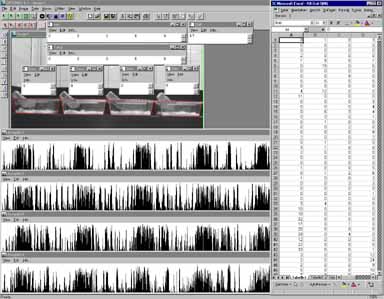
In our lab this method is used to record activity of individually housed mice for five consecutive days. By means of this technique the intensity (number of active seconds per minute) and the duration (number of minutes with at least one active second) of the activity could be measured for four individuals at a time (Fig. 10).
Digital image processing has become a viable tool for automatization of tests in animal behavior. Especially for frequently used tests to analyze rodent behavior like the open-field test, the elevated plus-maze test, etc. automatization by means of digital imaging has become indispensable. Every experimenter who finds himself/herself in the situation of testing hundreds of mice, as it is sometimes requested for example in behavioral phenotyping of gen targeted mice (e.g. 7), highly appreaciates the commodities that come along with automatization. Apart from the fact that "manual" scoring of large numbers of animals is very time consuming, this technique allows to gather information of higher quality due to better "fine tuning". Moreover, automated data collection allows to reduce the experimenter variability to a minimum degree (8). However, one should bear in mind that the establishment of an automated system has to include a thorough evaluation of the system by means of comparing the automatically gathered data to scores that were manualy recorded. Although automatization facilitates data collection in large numbers of tests, it is not suitable for all kind of behavior recording especially when complex behavioral patterns or interactions of animals are the object of research. Hence, automatization does not suffice to completely replace a trained eye of an experienced observer.
Acknowledgement This work was supported by a grant from the Deutsche Forschungsgemeinschaft (Sa 389/5) to Norbert Sachser.References 1: Altmann J. (1974): Observational Study of Behavior: Sampling Methods. Behaviour 49, 227-267. 2: Martin P. & P. Bateson (1993): Measuring Behaviour: An introductory guide. 2nd edition. Cambridge: Cambridge University Press. 3: Caro T.M., Roper R., Young M. & G.R. Dank (1979): Interobserver reliability. Behaviour 69, 303-315. 4: Schoenherr S.E.: The Evolution of the Computer. From:http://history.sandiego.edu/gen/recording/computer1.html. 5: Mandelbrot B. (1977): The Fractal Geometry of Nature. New York: W.H. Freeman. 6: Weisstein E.W.: Geometric Centroid. From: http://mathworld.wolfram.com/GeometricCentroid.html. 7: Lewejohann L., Skryabin B.V., Sachser N., Prehn C., Heiduschka P., Thanos S., Jordan U., Dell'Omo G., Vyssotski A.L., Pleskacheva M.G., Lipp H.-P., Tiedge H., Brosius J. & H. Prior (2004): Role of a neuronal small non-messenger RNA: behavioural alterations in BC1 RNA-deleted mice. Behavioural Brain Research. 8: Lewejohann, L; Reinhard, C; Schrewe, A; Brandewiede, J; Haemisch, A; Görtz, N; Schachner, M; Sachser, N (2006): Environmental Bias? Effects of Housing Conditions, Laboratory Environment, and Experimenter on Behavioral Tests. Genes Brain and Behavior 5: 64-72. |
Scholarly reference to this article should be like: Lewejohann, L (2004): Digital Image Processing in Behavioral Sciences. http://www.phenotyping.com/digital-image-processing.html.